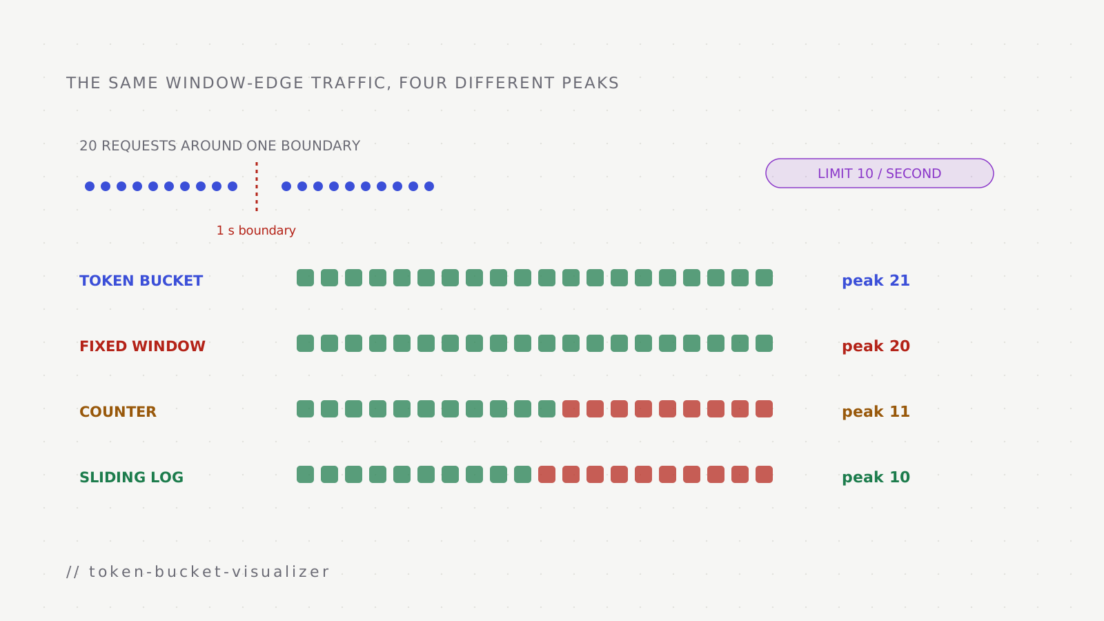
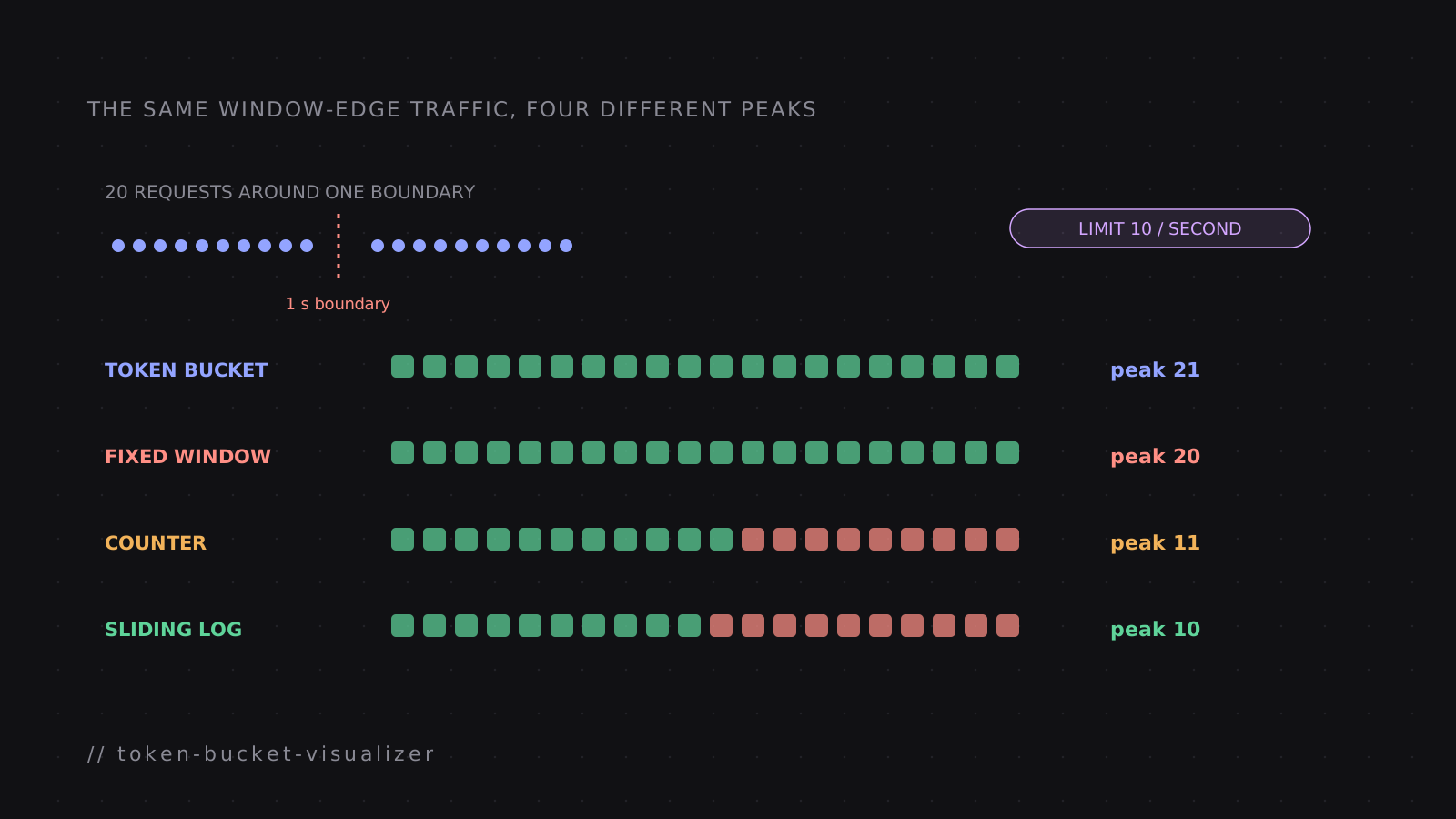
A service promises to accept 10 requests per second. At 5.0 seconds, twenty requests arrive around a one-second boundary. Does “10 per second” mean ten pass, twenty pass, or some burst in between? The answer depends on the algorithm and the exact times it remembers.
This simulator sends the same repeatable traffic to four algorithms. In a service running on several application instances, a shared counter store keeps all instances on one budget. The simulator can make that store unavailable from 20 to 30 seconds, so each outage policy becomes visible as allowed and rejected requests rather than a label in configuration.
How to read the diagrams
- Requests admitted
- Requests refused
- The shared store is unavailable
- Tokens available for a future request
A guided first run
Use the default limit of 10 req/s, meaning ten requests per second, and a
bucket size of 20 tokens. Each control updates the same sixty-second run
immediately.
Learn the normal case
- Leave Shared store on No outage and Show algorithm on Token bucket. At 15 seconds, compare the tall request bar with the falling token line below it.
- Read Peak in any 1 s as the most pressure the service receives in any moving one-second interval. With the defaults, token bucket peaks at 25 while the exact sliding log peaks at 10.
Expose the trade-offs
- Change Traffic to Window edges. Exactly ten requests arrive on each side of the boundary; compare the fixed window with the two sliding algorithms.
- Choose Runaway 6×, then compare Local full limit ×4 with Local share ÷4. The amber band shows how the same outage traffic gets a very different budget.
Requests per 200 ms · Token bucket
Horizontal axis: time from 0 to 60 seconds. Vertical axis: 0 to 5 requests in each 200 ms interval.
Tokens in the bucket
Horizontal axis: time from 0 to 60 seconds. Vertical axis: 0 to 20 available tokens.
Dashed line: the bucket's capacity of 20 tokens. It refills at 10 tokens a second.
| Algorithm | Peak in any 1 s | Allowed | Rejected |
|---|---|---|---|
| Token bucket | 25 (2.5×) | 319 | 41 |
| Fixed window | 14 (1.4×) | 305 | 55 |
| Sliding window counter | 9 | 303 | 57 |
| Sliding log (exact) | 10 | 305 | 55 |
The horizontal axis always covers 0–60 seconds. The request chart's vertical axis counts requests in each 200 ms bar and changes scale with the selected traffic; a triangle marks a bar that extends above the visible scale. The dashed line converts the per-second limit into the equivalent amount for one 200 ms bar. Green requests pass, red requests are refused, and the amber band is the ten-second store outage.
The table runs all four algorithms over the same arrivals. “Peak in any 1 s” uses a moving one-second interval, so it describes the largest short-term load delivered downstream. Totals answer a different question: how much traffic passed across the full minute.
The four algorithms
Token bucket
A bucket has a capacity and a refill rate. Each admitted request spends one token. With a capacity of 20 and a refill rate of 10 tokens per second, an idle service starts with 20 tokens: 20 requests arriving together can pass, request 21 is refused, and five tokens return after half a second. The capacity is therefore a burst allowance, while the refill rate controls the long-run pace.
The simulator's Quiet, then a burst pattern also sends background traffic, so its default moving peak is 25 rather than exactly 20. Watch the token line: saved tokens fund the front of the burst, then new requests wait for refills.
Fixed window
A fixed window stores one counter for a named interval such as second 4 or second 5. Give each interval a limit of 10. If ten requests arrive from 4.9–5.0 seconds and another ten arrive from 5.0–5.1, both counters remain within their own limit. The protected service receives 20 requests across 200 ms.
This is the boundary problem. It does not mean every fixed-window run permits twice the limit; traffic must bunch on both sides of the reset. The Window edges preset creates that condition and the fixed-window row reports a peak of 20 at the default rate.
Sliding window counter
The counter approximation keeps the previous fixed-window count and the current count. It weights the previous count by how much of that window still overlaps the last second. If the previous count is 10 and the new window is 20% complete, the estimate begins at 10 × 0.8 + 0 = 8. Two requests can pass before the estimate reaches 10.
The estimate needs constant storage and smooths the hard reset, but it does not remember exact request times. This simulator applies the same admission rule as the Lua in the companion article: the request passes only when estimate + 1 <= limit. Any difference from the exact log therefore comes from the approximation, rather than from a looser comparison.
Sliding log
The exact log stores one timestamp for every admitted request. Before checking a new request, it removes timestamps older than one second and counts what remains. If ten timestamps fall between 0.2 and 0.9 seconds, a request at 1.0 is refused because all ten are still inside the moving interval. After the earliest timestamp leaves the interval, one place becomes available.
That precision costs memory and cleanup work proportional to admitted traffic. With the shared store available, it is the reference behavior: the Peak in any 1 s value does not exceed the configured limit. During a fail-open outage, the policy bypasses every algorithm, including the sliding log.
- algorithm
- Token bucket
- known use
- APIs that allow a documented burst above a sustained rate
- cost of that choice
- Stores a small amount of state, but burst capacity must be chosen deliberately
- algorithm
- Fixed window
- known use
- Simple counters and coarse quotas
- cost of that choice
- Two adjacent windows can admit almost twice the nominal rate in a short interval
- algorithm
- Sliding counter
- known use
- Distributed limits that need a smoother boundary with constant storage
- cost of that choice
- The weighted count is an estimate
- algorithm
- Sliding log
- known use
- Low-volume limits where exact recent timestamps matter
- cost of that choice
- Storage and cleanup grow with admitted traffic
What changes when the shared store disappears
The normal algorithms assume every service instance reads and updates one shared state. Seconds 20–30 can replace that check with one of three policies. The longer article, Your Rate Limiter Will Fail Open or Closed, explains how to choose among them by protected resource.
- policy
- Fail open
- what seconds 20–30 do
- Admit every arrival while the store is unavailable
- default steady-overload result
- 150 of 150 outage requests pass
- policy
- Fail closed
- what seconds 20–30 do
- Refuse every arrival while the store is unavailable
- default steady-overload result
- 0 of 150 outage requests pass
- policy
- Local full limit ×4
- what seconds 20–30 do
- Give all four instances the full global rate and capacity
- default steady-overload result
- Availability stays high, but aggregate budget can grow fourfold
- policy
- Local share ÷4
- what seconds 20–30 do
- Give each instance one quarter of the global rate and burst capacity
- default steady-overload result
- Aggregate budget stays near the target under even distribution
Full-limit local fallback has four times the configured refill budget because all four instances refill at the global rate. Each also starts the outage with a full bucket. The divided-share option models the common mitigation: each instance receives global rate ÷ instance count and global burst ÷ instance count. That keeps the aggregate close to the target only while traffic is spread evenly and the instance count is current. Uneven load can still empty one local bucket while another has tokens.
Further experiments
Set the bucket size to 1 under Quiet, then a burst. This changes two things together: the bucket can save only one token, and the generated burst shrinks because that preset defines its burst as three times the selected capacity. The token bucket still drops excess traffic; it does not queue and release requests later as a traffic shaper would.
Raise the bucket size without changing the limit. The long-run rate stays at 10 requests per second, while the one-second peak grows because more credit can accumulate. This separates two controls that are often treated as one number.
Under Steady overload, compare fail open and fail closed by the “Allowed in outage” column. Both policies are internally consistent, yet they move the entire failure to different systems: fail open sends 150 requests downstream in this run; fail closed rejects all 150 at the edge.
What the simulation leaves out
Every request costs one unit here. A production limiter may charge more for an expensive export than a cached read. The shared store has only “up” and “down” states; latency, timeouts and partial errors are absent. Both local fallbacks distribute requests evenly across four fixed instances, while real load balancers and autoscalers change the distribution. Refused clients do not retry, so the generated traffic never reacts to a 429 response.
The model also treats the configured rate as an integer request count inside one-second windows. It is a teaching tool for algorithm behavior and failure policy, rather than a performance model for a particular Redis deployment.